UAB Galaxy RNA Seq Step by Step Tutorial
https://docs.rc.uab.edu/
Please use the new documentation url https://docs.rc.uab.edu/ for all Research Computing documentation needs.
As a result of this move, we have deprecated use of this wiki for documentation. We are providing read-only access to the content to facilitate migration of bookmarks and to serve as an historical record. All content updates should be made at the new documentation site. The original wiki will not receive further updates.
Thank you,
The Research Computing Team
Transcriptome analysis via RNA-Seq
There are several types of RNA-Seq: transcriptome, splice-variant/TSS/UTR analysis, microRNA-Seq, etc. This tutorial will focus on doing a 2 condition, 1 replicate transcriptome analysis in mouse.
Background
Web Resources
- Jeremy Goecks' Galaxy RNAseq tutorial http://main.g2.bx.psu.edu/u/jeremy/p/galaxy-rna-seq-analysis-exercise
- Tophat short-read RNA mapper http://tophat.cbcb.umd.edu/
- Cufflinks transcript assembler http://cufflinks.cbcb.umd.edu/
- Tophat-cuff[links,compare,diff] tutorial (command-line) http://cufflinks.cbcb.umd.edu/tutorial.html
- IGV (Broad Integrated Genome Viewer) http://www.broadinstitute.org/software/igv/download
- IGB (Integrated Genome Browser) http://bioviz.org/igb/download.shtml
- UCSC Genome Browser http://genome.ucsc.edu/
File Types and Acronyms
- FASTQ - text file; like a FASTA but with extra lines for read quality scores for each base. This is what you usually get from the sequencing center.
- BAM - Binary compresssed sequences Alignment/Map format - Contains a copy of the reference genome, and every short read that was mapped, including the short reads location and alignment. It can also contain the "left-over" reads from the source FASTQ's that did NOT align to the reference genome! These files must visualized with a tool, either IGV, IGB or sometimes UCSC Genome Browser.
- BED - text file; a list of locations, in genomic coordinates.
- GTF Gene Transfer Format - text file; contains gene/transcript annotations for a sequence/genome, also in genomic coordinates.
- FASTA - text file; contains a list of named sequences. Can be used to hold the sequence of a reference genome to which RNAseq reads will be mapped.
- FPKM (RPKM) - acronym; Fragments Per Kilobase of exon per Million fragments mapped
Upload data
For this tutorial, we will have 2 mouse samples, sequenced with paired-end reads on an Illumina machine. That gives us 4 FASTQ files to upload (forward and reverse sequences for each sample).
FTP site for compressed fastq.gz files
- control_mm9_chr15_Plekhh2-PigF_forward.fastq.gz
- control_mm9_chr15_Plekhh2-PigF_reverse.fastq.gz
- drugged_mm9_chr15_Plekhh2-PigF_forward.fastq.gz
- drugged_mm9_chr15_Plekhh2-PigF_reverse.fastq.gz
Or they can be found inside Galaxy at Shared Data / Data Libraries / Tutorial Data Sets / RNAseq Tutorial
Set filetype and genome
To start, you must move the data (FASTQ) from the sequencing center into the Galaxy instance, be sure to specify the filetype ("fastqsanger" for UAB and HudsonAlpha, the default "fastq" will not work) and the organism that was sequenced ("Genome database"), in this tutorial, "mm9" for mouse.
Check quality of READ data
At this step, we check the quality of sequencing. This was already covered in the DNA-Seq tutorial, under Galaxy_DNA-Seq_Tutorial#Assessing_the_quality_of_the_data Assessing the quality of the data. This says nothing about the quality of the sample, or whether it was the right sample. We'll check that later.
At a minimum, for each FASTQ file, run NGS: QC and manipulation > FASTQ QC > Fastqc
This quick tool will give you a nice HTML report, including dashboard summary. If some of the reports are not green, discuss this with your sequencing center.
In some cases, you may need to trim bases off the beginning or ends of the sequence. See the tools in NGS: QC and manipulation > FASTX-TOOLKIT FOR FASTQ DATA.
Align using TopHat
For the moment, TopHat is the standard NGS aligner for transcript data, as it handles splicing. In addition, it can be set to detect indels relative to the reference genome.
We'll run TopHat once for each sample (twice, in this case), providing it with 2 FASTQ files each time (forward and reverse reads).
Menu: NGS: RNA Analysis > Tophat for Illumina
Tophat Inputs
- Reads (FASTQs)
- FASTQs As we're doing "paired" reads, we will need to provide 2 FASTQ files: the forward and reverse reads. In order to have a place to specify the 2nd FASTQ file, we must set the "Is this library mate-paired?" pulldown to "Paired-end", then a second pulldown will appear to specify the 2nd FASTQ.
- Mean Inner Distance between Mate Pairs is a value you must get from your sequencing center. This is the mean fragment length of the molecules sequenced, minus the part sequenced. For many RNAseq experiments, it is around 150-175.

- Genome (Built-in or FASTA from history)
- We must provide it with the reference genome to align to. In our case, this is Mouse, and we'll use the already installed "mm9" genome build. If you have an genome that is not on the list, you can either have us add it, or you can upload a FASTA file of the genome into your history, and point TopHat at that.
- TopHat settings to use
- Defaults
- This is the easy thing to do, but, as the manual said, "There is no such thing (yet) as an automated gearshift in splice junction identification. It is all like stick-shift driving in San Francisco. In other words, running this tool with default parameters will probably not give you meaningful results."
- Full parameter list
- The most common thing to change
- Allow indel search (from NO to YES)
- Minimum isoform fraction (to 0 if looking for rare isoforms)
- Maximum/minimum intron length (defaults are for Mammals; other critters will do better with stricter settings)
- The most common thing to change
TopHat output
- accepted_hits (BAM, BAI)
- Two binary files: .BAM (data) and .BAI (index)
- These are the actual paired reads mapped to their position on the genome, and split across exon junctions. This can be visualized in IGV, IGB or UCSC, but you must download both .BAM and .BAI files to the same directory.
- splice_junctions (BED)
- BED file (list of genomic locations, no sequence) listing all the places TopHat had to split a read into two pieces to span an exon junction. This can be visualized at UCSC or in IGV, etc.
- deletions (BED) (if indel search is on)
- insertions (BED) (if indel search is on)
Alignment/Mapping QC
Next we check the quality of the TopHat mapping to the reference genome. This will detect not only problems with the sequencing runs, but also contamination or swapping of the samples.
For each sample, run NGS: SAM Tools > flagstat on the accepted_hits.bam file from tophat. While the same tool is used to assess the output of other short-read genomic aligners (BWA, bowtie, etc), the values are interpreted a little differently.
 # flagstat output
 28316 in total # ignore
 0 QC failure
 0 duplicates
 28316 mapped (100.00%) # ignore
 28316 paired in sequencing
 14258 read1
 14058 read2
 16398 properly paired (57.91%) # important value!
 28010 with itself and mate mapped
 306 singletons (1.08%)
 0 with mate mapped to a different chr
 0 with mate mapped to a different chr (mapQ>=5)
Things to ignore
- in total and mapped (100.00%): these numbers always match and give 100% for tophat runs.
- The in total can also be greater than the number of reads in the original FASTQ, as tophat can create multiple matches for a read.
Things to look at
- properly paired should be above 50%, the higher the better. This is the count of read-pairs (sequences from the opposite ends of the same physical fragment) that mapped within the expected distance of each other, and in the expected orientation. Ideally this should be 100%.
- If properly paired is low the mapping quality may be bad, or there may be sample contamination.
- If very few reads map, take 500-1000 random un-mapped reads from your FASTQ file, and use NCBI Megablast(n), then request a taxonomy report (metagenomics!). This will tell you if your mouse sample was swapped with someone else's human one, or if your yeast sample was overgrown with bacteria.
Visual Inspection - you should also download the BAM/BAI file pair and visualize it in IGV or IGB, to see if it looks reasonable.
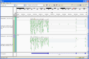
Tophat.accepted_hits viewed in IGV

Construct transcripts using Cufflinks
Cufflinks takes the mapped reads for each sample and tries to reconstruct the individual transcripts and isoforms. This can be done "de novo", without using any previous gene annotations, limited strictly to only computing expression levels of existing annotations, or a combination of the two.
For this exercise, we are comparing transcription levels between treatment samples, so we are primarily interested in known genes. However, it is always wise to keep an eye out for something new, so we'll use the combination mode. That will give us accurate values for annotated transcripts/genes, but still allow discovery of novel phenomenon.
Menu: NGS: RNA Analysis > Cufflinks Run once for each sample.
Cufflinks inputs
- Mapped Reads (SAM or BAM)
- SAM or BAM file of aligned RNA-Seq reads: use accepted_hits.bam from tophat
- Genome annotation (GTF)
- Use Reference Annotation = yes, then you get a 2nd pulldown Reference Annotation where you can choose a GTF file from your history. In order to get gene NAMES, and not just accession numbers, use the modified GTF files in the Shared Data > Data Libraries > Patched GTF annotation files for Cufflinks
- Other Parameters
- Perform quartile normalization
- normally use YES, but for this exercise use NO, because we're not working with a full genome's worth of reads and the statistics will go haywire.
- Perform Bias Correction
- normally use YES, but for this exercise use NO, because we're not working with a full genome's worth of reads and the statistics will go haywire.
Cufflinks outputs
- assembled transcripts (GTF)
- all isoforms with their exon structure and expression levels. We'll use this for the next steps.
- transcript_expression (tabular)
- table of expression levels for each transcript
- gene_expression (tabular)
- table of total expression levels for each gene.
If we did not have multiple conditions, we could stop here.
Cufflinks QC
- Check that all the FPKM values in these files are not zero.
- Check that the gene symbols show up where you want them. If all the gene_id's are "CUFF.#.#", it will be hard to figure things out.
- Visualize assembled_transcripts
Track and Assemble Transcripts with CuffCompare
To simply get gene/transcript expression differences of known genes between samples, this step can be skipped. However, if you want to include any novel genes detected in your analysis, you need this.
Cuffcompare is not well named, it should be something more like cuffCorrelate. It determines which transcripts are the same across a set of samples, and builds the mapping tables. Importantly for our purposes, it also builds combined_transcripts.gtf which lists every transcript seen in ANY sample. It can also compute the differences between the observed transcript annotation and the "official" one.
Depending of your reference GTF annotation file, cuffcompare also performs the function of creating p_id (protein id) and tss_id (transcription start site id) which will be needed by cuffdiff later. Because the new GTFs from the iGenomes project include these needed attributes by default. However, if you download a gene annotation file directly from Ensembl/UCSC (rather than using one from iGenomes), you'll need to use Cuffcompare in the process to get a GTF file that can used by Cuffdiff.
cuffcompare inputs
- assembled_transcripts for each sample
- Enter the assembled_transcript files from the cufflinks run for each experiment. You will need to repeatedly click Add new Additional GTF Input Files in order to get additional chooser boxes to select all the GTFs.
- Use Reference Annotation
- Set this to yes and a pulldown, Reference Annotation, will appear. This will be our patched genomic GTF file.
cuffcompare outputs
- combined_transcripts.gtf
- For this exercise, we only use this one output, which will be the augmented genome annotation we'll use in our final step, cuffdiff.
Fold Change Between Conditions: CuffDiff
Cuffdiff does the real work determining differences between experimental conditions. In our case, we have two conditions (control, drugged), with 1 replicate each. However, cuffdiff can handle many conditions, each with several replicates, in one go.
cuffdiff inputs
- Model
- Transcripts should be the combined_transcripts.gtf from our cuffcompare run. If we really don't care about novel genes, and skipped the cuffcompare step, we use the patched genomic gtf file (mm9_RefGene_patched3.gtf) that we originally gave to tophat!
- Mapped Read Data
- perform replicate analysis should ALWAYS be yes.
- When you turn this on, you can created named groups for each condition. While it less clicking not to use this for the basic case (2 conditions, 1 replicate each), if you don't use this, then your groups will not be named in your output files. If you do use this, your output files will be much easier.
- Create a group for each condition. In our case, "control" and "drugged".
- Add replicates to each group. In our case, 1 replicate per group/condition. The replicates are the mapped reads from tophat in the accepted_hits.bam files.
- Thresholds for reporting
- False Discovery Rate thresholds what gets flagged as "significant".
- Min Alignment Count thresholds how many reads a transcript needs to given an "OK" status, instead of "NOTEST".
- Statistical enhancements
- Perform quartile normalization Normally 'yes, but for our example NO, because we don't have full genome coverage, and the statistic would go wild.
- Perform Bias Correction Normally 'yes, but for our example NO, because we don't have full genome coverage, and the statistic would go wild.
cuffdiff outputs
Cuffdiff has many, many output files. What you focus on will depend on what biological questions you are interested in:
- TSS... files report on Transcription Start Sites
- splicing... report on splicing
- CDS... track coding region expression
- transcript... track
- gene... rolls up the transcripts into their genes.
For our simple example, we'll just look at changes in transcript expression.
- gene/transcript FPKM tracking (tabular)
- gives information about the gene/transcript (length, nearest_ref_id=NM_#####, TSS, etc) and the confidence intervals for FPKM for each condition.
- gene/transcript differential expression testing (tabular)
- gives the expression change between groups, a status of whether there was enough data for that value to be accurate (OK is good, FAIL and NOTEST are bad. LOWDATA is somewhere in between). Finally, it gives a p-value.
extracting the data you want
So, some info we want (nearest_ref_id) is in one file, while the rest is in the other. We'll use Galaxy tabular data tools to merge the two files, and filter down to what we want. You could do this by hand in Excel, and probably a lot faster the first time. But once you figure out how to do it once in Galaxy, you can save that "workflow" and re-use it again later!
- join transcript_FPKM_tracking to transcript_differential_expression_testing based on tracking.tracking_id=testing.test_id.
- Join, Subtract and Group > Join two Datasets, specify using column as c1 in both cases.
- join lost the headers, so we'll extract those from the original files and stick them back on the front
- Text Manipulation > Select first, and set lines to 1, and from to transcript_FPKM_tracking
- Text Manipulation > Select first, and set lines to 1, and from to transcript_differential_expression_testing
- Text Manipulation > Paste, and choose transcript_FPKM_tracking and transcript_differential_expression_testing
- Text Manipulation > Concatenate datasets, and choose the Paste results (headers), then the Join results (data)
- narrow this down to the columns we want to look at
- Text Manipulation > Cut - allows you to map from one set of columns to new set. You can leave out columns, duplicate columns and change column order. Very versatile tool! - Cut the columns "c1,c3,c5,c7, c23, c21, c24, c22, c25, c26, c28".
- then select just the rows we want (can use formulas or regexs)
- Filter and Sort > Filter with the condition c5=='OK' or c5 == 'LOWDATA' or c5=='status, where the last term keeps the header around.